User:Sidharth

Tabulated frontend to FPROPS

Author of the page Sidharth Somanathan is a GSOC (Google Summer Of Code) 2015 participant. During the summer of 2015 he was also a PhD candidate in Physics at Texas A&M University. His interests in general are in algorithms and parallel computing.

Link to fprops folder in his subversion branch where the code was added --> sid/models/johnpye/fprops/:/

External link to the GSOC 2015 project page --> [1]

Theory

Finding a property X at <math> (T,\rho) </math> provided we know value of X and its first and second order derivatives at a nearby point <math> (T_i,\rho_j) </math>

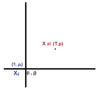
We intend to implement a tabulated frontend to the existing FPROPS. The main idea for this comes from the Tabulated Taylor Series Expansion (TTSE) approach. We would make a 2 dimensional grid in temperature and mass density <math> (T,\rho) </math>. The essence of the approach is that if we know the value of a thermodynamic property <math> X </math> and its first, second and mixed derivative terms with respect to two independent variables <math> (T,\rho) </math> at a certain point <math> (T_i,\rho_j) </math> then we can compute the value of the function at a small distance from the point by the following Taylor series expansion.

<math> X = X_{i,j} + (T-T_i) \frac{\partial X}{\partial T}\bigg|_{i,j} + \frac{1}{2} (T-T_i)^2 \frac{\partial^2 X}{\partial T^2}\bigg|_{i,j} + (\rho-\rho_j) \frac{\partial X}{\partial \rho}\bigg|_{i,j} + \frac{1}{2} (\rho-\rho_j)^2 \frac{\partial^2 X}{\partial \rho^2}\bigg|_{i,j} + (T-T_i) (\rho-\rho_j) \frac{\partial^2 X}{\partial T \partial \rho}\bigg|_{i,j} </math>

Here X could be thermodynamic properties like pressure, enthalpy etc. For implementing this we can allocate a 200×200 grid with each of the six terms in the above equation for the key state properties we need, namely <math>(p, h, s) </math>. In order to do this, the back-ends (eg Helmholtz, Peng-Robinson) need to be supplemented with additional routines, to compute the first and second order derivatives. For instance for entropy expansion we need

<math> \frac{\partial s}{\partial T}\bigg|_{\rho} , \frac{\partial^2 s}{\partial T^2}\bigg|_{\rho} , \frac{\partial s}{\partial \rho}\bigg|_{T} , \frac{\partial^2 s}{\partial \rho^2}\bigg|_{T} </math> and <math> \frac{\partial^2 s}{\partial \rho \partial T} </math>

FPROPS module in ASCEND

FPROPS uses function pointers from the underlying correlation (helmholtz or Pengrob) to calculate fundamental quantities with Temperature and <math> \rho</math> as the input. Following are those functions of fprops :-

fprops_p() fprops_u() fprops_h() fprops_s() fprops_g()
fprops_dpdrho_T() fprops_alphap() fprops_betaP() fprops_a()
fprops_cp() fprops_cv() fprops_w()


Both the underlying correlations provide these 13 functions calculated from first principles, with T and <math>\rho</math> as inputs. So the TTSE implementation for a specific liquid and a specific correlation (H or P) should eventually generate tables for each of the above 13 entries. For the saturation function fprops_sat(), takes only 1 input (temperature) and returns saturated liquid density, saturated vapour density and the saturation pressure. This function involves solving equations iteratively and tabulation should speed up calculation on saturation curve.

To begin with we can tabulate the following functions:

• helmholtz_p
• helmholtz_s
• helmholtz_u
• helmholtz_g
• helmholtz_h

In order to use look up tables for TTSE method inside these routines we need to complete the set of all partial derivatives we need :-

For each of the above variable X (where X is either of P,s,u,g and h) we need <math> \frac{\partial X}{\partial T}\bigg|_{\rho} ,

\frac{\partial^2 X}{\partial T^2}\bigg|_{\rho} ,
   \frac{\partial X}{\partial \rho}\bigg|_{T} , 
\frac{\partial^2 X}{\partial \rho^2}\bigg|_{T}</math>   and <math>
  \frac{\partial^2 X}{\partial \rho \partial T} </math>

Many of the partial derivatives are already listed in helmholtz.c. Specifically the new 18 ones we need to implement are:

Table 1

Variable	Partial derivative with T constant	Partial derivative with <math>\rho</math> constant	Partial second derivative with <math>\rho</math> constant	Partial second derivative with <math>T</math> constant	Partial mixed second derivative
Pressure, P	<already implemented>	<already implemented>	<already implemented>	helmholtz_d2pdT2_rho() <math>\frac{\partial^2 p}{\partial (T^2)} </math>	helmholtz_d2pdrhodT() <math>\frac{\partial^2 p}{\partial (T \rho)} </math>
Enthalpy, h	<already implemented>	<already implemented>	helmholtz_d2hdrho2_T() <math>\frac{\partial^2 h}{\partial \rho^2}\bigg|_{T}</math>	helmholtz_d2hdT2_rho() <math>\frac{\partial^2 h}{\partial T ^2}\bigg|_{\rho}</math>	helmholtz_d2hdrhodT() <math>\frac{\partial^2 h}{\partial (T \rho)} </math>
Internal Energy, u	<already implemented>	<already implemented>	helmholtz_d2udrho2_T() <math>\frac{\partial^2 u}{\partial \rho^2}\bigg|_{T}</math>	helmholtz_d2udT2_rho() <math>\frac{\partial^2 u}{\partial T^2}\bigg|_{\rho}</math>	helmholtz_d2udrhodT() <math>\frac{\partial^2 u}{\partial (T \rho)}</math>
Entropy, s	helmholtz_dsdT_rho() <math>\frac{\partial s}{\partial T}\bigg|_{\rho}</math>	helmholtz_dsdrho_T() <math>\frac{\partial s}{\partial \rho}\bigg|_{T}</math>	helmholtz_d2sdrho2_T() <math>\frac{\partial^2 s}{\partial \rho^2}\bigg|_{T}</math>	helmholtz_d2sdT2_rho() <math>\frac{\partial^2 s}{\partial T^2}\bigg|_{\rho}</math>	helmholtz_d2sdrhodT() <math>\frac{\partial^2 s}{\partial (T \rho)}</math>
Gibbs Free Energy, g	helmholtz_dgdT_rho() <math>\frac{\partial g}{\partial T}\bigg|_{\rho}</math>	helmholtz_dgdrho_T() <math>\frac{\partial g}{\partial \rho}\bigg|_{T}</math>	helmholtz_d2gdrho2_T() <math>\frac{\partial^2 g}{\partial \rho^2}\bigg|_{T}</math>	helmholtz_d2gdT2_rho() <math>\frac{\partial^2 g}{\partial T^2}\bigg|_{\rho}</math>	helmholtz_d2gdrhodT() <math>\frac{\partial^2 g}{\partial (T \rho)}</math>

To evaluate these drivatives we need the underlying partial derivatives of the residual and the ideal part of helmholtz function. So the three new functions needed in helmholtz.c and cp0.c

Third partial derivative of ideal part of helmholtz (all other partial derivatives invloving delta are zero) in file cp0.c

• ideal_phi_tautautau()

Third derivative of helmholtz residual function, with respect to delta once and tau twice

• helm_resid_deltautau()

Third derivative of helmholtz residual function, with respect to delta twice and tau once

• helm_resid_deldeltau()

Third derivative of helmholtz residual function, with respect to tau thrice

• helm_resid_tautautau()

Two Phase

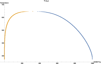
Saturation dome derived from helmholtz_sat().When the input temperature is between <math>T_t</math> and <math>T_c</math> we see the mixed states with both <math>\rho_f</math> and <math>\rho_g</math> computed by the function until they meet at <math>T_c</math>. The yellow points are for the fluid density and the blue points are for gaseous density of the mixed phase.

For temperature's lying between Tt and Tc the fluid is in mixed phase.

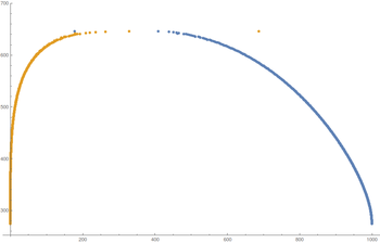
Saturation dome derived from evaluate_ttse_sat().Like the previous plot the yellow points are for the fluid density and the blue points are for gaseous density of the mixed phase. We can see the significant errors close to Tc.

For temperature's lying between Tt and Tc the fluid is in mixed phase.

fprops_sat_T() deals with the saturation condition when the input temperature lies between Tt and Tc. It uses iterative procedure to find <math>\rho_f</math> and <math>\rho_g</math> to find the proportion of fluid and gas in the mixture. Here we can achieve speed-up if we do a fit on both sides(liquid and vapor sides) of saturation dome. For this we can do Taylor series expansion of <math>\rho_f(T) </math> and <math>\rho_g (T)</math> with respect to temperature.

<math> \rho = \rho_{i,j} + (T-T_i) \frac{\partial \rho }{\partial T}\bigg|_{i,j} + \frac{1}{2} (T-T_i)^2 \frac{\partial^2 \rho }{\partial T^2}\bigg|_{i,j} </math>

The function evaluate_ttse_sat() is used to find <math>\rho_f</math> and <math>\rho_g</math> now, using the tables previously created with helmholtz_sat(). The Taylor expansion mentioned above is used to calculate the <math>\rho_f</math> and <math>\rho_g</math> at off-grid values.

The two plots to the right show the comparison between Helmholtz calculated curve and the table calculated curve.

---

Preliminary Results

In this test the fluid of choice was taken to be water. We need boundaries for the table implementation in <math>(T,\rho)</math> plane. So for this test <math> (T_{min}, T_{max}) </math> was taken to be (200,4200) K and <math>(\rho_{min}, \rho_{max})</math> was taken to be (400,4400) kg/m³. This domain was decomposed into 200×200 points.

The test was also done for a first order implementation of TTSE, in which we just take the below first order formulation.

<math>

X = X_{i,j} + (T-T_i) \frac{\partial X}{\partial T}\bigg|_{i,j} + (\rho-\rho_j) \frac{\partial X}{\partial \rho}\bigg|_{i,j} </math>

For this particular test <math> \rho </math> was set to <math> \mathbf{200} </math> Kg/m^3 and temperature is ranged from <math> \mathbf{400}</math> Kelvins to <math> \mathbf{500} </math> Kelvins in <math> \mathbf{500} </math> equal steps. And then the five functions given below (and implemented in ttse.c) are called for the tabulated result and compared with the direct helmholtz result

evaluate_ttse_p() //for pressure
evaluate_ttse_h() //for enthalpy
evaluate_ttse_s() //for entropy
evaluate_ttse_u() //for internal energy
evaluate_ttse_g() //for Gibbs free energy


Comparing time for building tables

	First Order	Second Order
Time In Seconds	6.231	16.096645

Comparing Average % Error for the five variables

	For First Order	For Second Order
Pressure	0.001419	0.000074
Enthalpy	0.000892	0.000009
Entropy	0.024706	0.000411
Internal Energy	0.005294	0.000125
Gibb's Energy	0.082597	0.086281

Run Time Comparison - Helmholtz V/S TTSE

TTSE based evaluation	Time In Seconds for 500X5 = 2500 computations	Speed Up
First order	1.130000e-04	180X
Second Order	1.380000e-04	146X

For a larger set of 5X100000 computations. Here the temperature ranges from 400 to 1200K in 100000 steps. For this set Helmholtz EOS took almost 3.92 seconds. Below is the time for first and second order TTSE calculation for same set.

Run Time Comparison - Helmholtz V/S TTSE

TTSE based evaluation	Time In Seconds for 500000 computations	Speed Up
First order	2.270700e-02	174X
Second order	2.500000e-02	156X

---

Progress Details

• Implemented all the 18 functions from Table 1 in helmholtz.c
• Implemented the above 4 functions for triple derivatives using a naive formulation from the second derivatives. Can be improved later.
• Added struct ttse in rundata.h. This contains the necessary information needed in structure.
• ttse.c and ttse.h file added to fprops/ . Here the TTSE module will be fully implemented.
• Testing module for TTSE added in test/test_ttse.c
• A simple test added in test/test_ttse.c for water fluid.
• TTSE integrated with helmholtz.c
• Code for two phase added.
• Code for database of files added, provision to load from database implemented if the file already exists.
• TTSE is invoked when fprops_fluid is called with corrtype = "ttse" and the underlying correlation is HELMHOLTZ_TYPE in eos.